Kernel Density Estimation: Predict KDE & Generate Data

Task: For a given data set X, predict its density function. Using the found density function generate new random data set Y and check the hypothesis that X and Y distributions are identical.
Method: Histogram data generation, Gaussian Kernel Density Estimation data generation, K-S testing of density integral.
Tutorial type: Algorithm oriented, written in Python
Requirements: Python >= 2.7.0, Numpy >= 1.6.0, Matplotlib 1.4.3

Intro

Here we find a usage for Kernel Density Estimation (KDE) in real situation - random data generation of the same PDF as given dataset. To achieve the the following steps are taken:

We load the dataset, analyze it with histograms
Produce a PDF using different KDE techniques
Check if generated data is the same distribution as given dataset

Data generation from Histogram

First we try how good is approach to generate data from normalized histogram. In the code below the following steps are taken: find histogram of given dataset, generate new data of given distribution, plot the results.

import numpy as np
import matplotlib.pyplot as plt

#import data
#conists of one column of datapoints as 2.231, -0.1516, 1.564, etc
data=np.loadtxt("dataset1.txt")

#normalized histogram of loaded datase
hist, bins = np.histogram(data,bins=100,range=(np.min(data),np.max(data)) ,density=True)
width = 0.7 * (bins[1] - bins[0])
center = (bins[:-1] + bins[1:]) / 2


#generate data with double random()
generatedData=np.zeros(1000)
maxData=np.max(data)
minData=np.min(data)
i=0
while i<1000:
    randNo=np.random.rand(1)*(maxData-minData)-np.absolute(minData)
    if np.random.rand(1)<=hist[np.argmax(randNo<(center+(bins[1] - bins[0])/2))-1]:
        generatedData[i]=randNo
        i+=1

#normalized histogram of generatedData
hist2, bins2 = np.histogram(generatedData,bins=100,range=(np.min(data),np.max(data)), density=True)
width2 = 0.7 * (bins2[1] - bins2[0])
center2 = (bins2[:-1] + bins2[1:]) / 2

#plot both histograms
fig, (ax1, ax2) = plt.subplots(ncols=2, nrows=1, figsize=(14, 8), sharex=True, sharey=True,)
ax1.set_title('Original data')
ax1.bar(center, hist, align='center', width=width2, fc='#AAAAFF')
ax2.set_title('Generated data')
ax2.bar(center2, hist2, align='center', width=width2, fc='#AAAAFF')

fig.savefig("Loaded_and_Generated_Data.jpg")

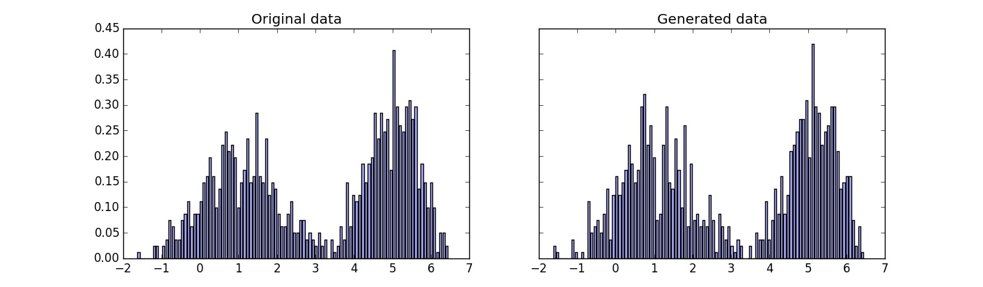
Visually distributions are very similar. We will evaluate the results precisely later, comparing it to data generated from Kernel Density Estimation.

Data generation using Kernel Density Estimation

Now the task is to find KDE first, then generate data from it. If you are not familiar with KDE take a look at this post explaining it. The following code uses Gaussian kernel and two methods to estimate optimal h: Silverman's and Least Squares Cross Validation (LSCV). The theory about LSCV can be found in this paper,

import numpy as np
import matplotlib.pyplot as plt

#https://en.wikipedia.org/wiki/Gaussian_function
def gaussian(x,b=1):
    return np.exp(-x**2/(2*b**2))/(b*np.sqrt(2*np.pi))
    
#import data
#conists of one column of datapoints as 2.231, -0.1516, 1.564, etc
data=np.loadtxt("dataset1.txt")

N=100 #Number of bins
lenDataset = len(data)
#normalized histogram of loaded datase
hist, bins = np.histogram(data, bins=N, range=(np.min(data), np.max(data)), density=True)
width = 0.7 * (bins[1] - bins[0])
dx=(bins[1] - bins[0])
center = (bins[:-1] + bins[1:]) / 2

##Generate data
#There are few options here - save values of KDE for every small dx 
#OR save all the dataset and generate probability for every x we will test.
#We choose the second option here.

sumPdfSilverman=np.zeros(len(center))
#Silverman's Rule to find optimal bandwidth
#https://en.wikipedia.org/wiki/Kernel_density_estimation#Practical_estimation_of_the_bandwidth
h=1.06*np.std(data)*lenDataset**(-1/5.0)

for i in range(0, lenDataset):
    sumPdfSilverman+=((gaussian(center[:, None]-data[i],h))/lenDataset)[:,0]
    
#So here we have to sum 1000 gaussians at generated random x to evaluate probability that this x exists in new generated dataset.
i=0
generatedDataPdfSilverman=np.zeros(1000)
while i<1000:
    randNo=np.random.rand(1)*(np.max(data)-np.min(data))-np.absolute(np.min(data))
    if np.random.rand(1)<=np.sum((gaussian(randNo-data,h))/lenDataset):
        generatedDataPdfSilverman[i]=randNo
        i+=1

#Our second approach to calculate optimal bandwidth h using least-squares cross validation
#This looks a bit tricky, take a look at the theory explanation in the related article if you need to.
h_test = np.linspace(0.01, 1, 100) #h values to iterate for testing
L = np.zeros(len(h_test))
fhati = np.zeros(len(data)) #fhati
center
iteration=0
for h_iter in h_test:
    #find first part of equation
    for i in range(0, lenDataset):
        fhat = 0
        fhat+=((gaussian(center[:, None]-data[i],h_iter))/lenDataset)[:,0]
    
    #find second part of equation for sum fhati
    for i in range (0, lenDataset):
        mask=np.ones(lenDataset,dtype=bool)
        mask[i]=0
        fhati[i]=np.sum(gaussian(data[mask]-data[i],h_iter))/(lenDataset-1)
    
    L[iteration]=np.sum(fhat**2)*dx-2*np.mean(fhati)
    iteration=iteration+1

h2=h_test[np.argmin(L)]
#we can look how L looks like, depending on h
fig0, ax0 = plt.subplots(1,1, figsize=(14,8))
ax0.plot(h_test,L)
fig0.savefig("Function_to_minimize[h,L_value].jpg")

#resulting PDF with found h2
sumPdfLSCV=np.zeros(len(center))
for i in range(0, lenDataset):
    sumPdfLSCV+=((gaussian(center[:, None]-data[i],h2))/lenDataset)[:,0]

#So here we have to sum 1000 gaussians at generated random x to evaluate probability that this x exists in new generated dataset.
i=0
generatedDataPdfCV=np.zeros(1000)
while i<1000:
    randNo=np.random.rand(1)*(np.max(data)-np.min(data))-np.absolute(np.min(data))
    if np.random.rand(1)<=np.sum((gaussian(randNo-data,h2))/lenDataset):
        generatedDataPdfCV[i]=randNo
        i+=1


##Plotting
fig, ax = plt.subplots(2,2, figsize=(14,8), sharey=True )
#Estimated PDF using Silverman's calculation for h
ax[0,0].plot(center, sumPdfSilverman, '-k', linestyle="dashed")
ax[0,0].set_title('KDE, Silvermans bandwidth h=%.2f' % h)

#Histogram for generated data using KDE and h found using Silverman's method
hist2, bins2 = np.histogram(generatedDataPdfSilverman, bins=N, range=(np.min(data), np.max(data)), density=True)
ax[1,0].bar(center, hist2, align='center', width=width, fc='#AAAAFF')
ax[1,0].set_title('Generated, Silvermans bandwidth h=%.2f' % h)

#Estimated PDF using Least-squares cross-validation for h
ax[0,1].plot(center, sumPdfLSCV, '-k', linestyle="dashed")
ax[0,1].set_title('KDE, LSCV bandwidth h=%.2f' % h2)

#Histogram for generated data using KDE and h found using LSCV
hist3, bins3 = np.histogram(generatedDataPdfCV, bins=N, range=(np.min(data), np.max(data)), density=True)
ax[1,1].bar(center, hist3, align='center', width=width, fc='#AAAAFF')
ax[1,1].set_title('Generated, LSCV bandwidth h=%.2f' % h2)

#note that PDF found using KDE does not sum up exactly to one, because we ignore the side-spread
#values produced by KDE
fig.savefig("Many_Points_Example_KDE.jpg")

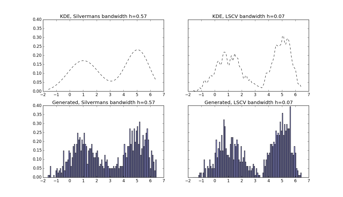
The above picture displays the output of the script. In top of it is the found PDF function using different bandwidth, found using different techniques. At the bottom the histograms of generated data with known PDF are displayed.

K-S Statistics To Evaluate If Generated Data Is The Same Distribution As Dataset

We will use the simple version of K-S statistics test described here, where we find maximum difference between cumulative PDF of two distributions - original and generated in our case.

Found D(difference) value is then compared against the table of critical values as shown in wikipedia article mentioned above. Consider the following code, showing how to compare every dataset we generated so far. One more important thing is the term Empirical distribution function, which is used in the theory. In fact it is the sum of histogram values divided by the count of total number of elements. We use normalized histograms here, so just need to multiply by dx.

cumulative = np.cumsum(hist)*dx               #original dataset
cumulativeHist = np.cumsum(hist1)*dx          #histogram generated
cumulativeKDE_Silverman = np.cumsum(hist2)*dx #KDE Silverman's h generated
cumulativeKDE_LSCV = np.cumsum(hist3)*dx      #KDE LSCV generated

DHist=np.max(np.absolute(cumulative-cumulativeHist))
DKDE_Silverman=np.max(np.absolute(cumulative-cumulativeKDE_Silverman))
DKDE_LSCV=np.max(np.absolute(cumulative-cumulativeKDE_LSCV))

fig, ax = plt.subplots(1,3, figsize=(16,4), sharey=True)
ax[0].set_ylim([0,1.4])
ax[0].plot(cumulative, label="Original data")
ax[0].plot(cumulativeHist, label="Histogram generated")
ax[0].legend()
ax[0].set_title('Dmax = %.3f' % DHist, y=0.05, x=0.7)

ax[1].plot(cumulative, label="Original data")
ax[1].plot(cumulativeKDE_Silverman, label="KDE_Silverman generated")
ax[1].legend()
ax[1].set_title('Dmax = %.3f' % DKDE_Silverman, y=0.05, x=0.7)

ax[2].plot(cumulative, label="Original data")
ax[2].plot(cumulativeKDE_LSCV, label="KDE_LSCV generated")
ax[2].legend()
ax[2].set_title('Dmax = %.3f' % DKDE_LSCV, y=0.05, x=0.7)

fig.savefig("Cummulative_sum_test.jpg")

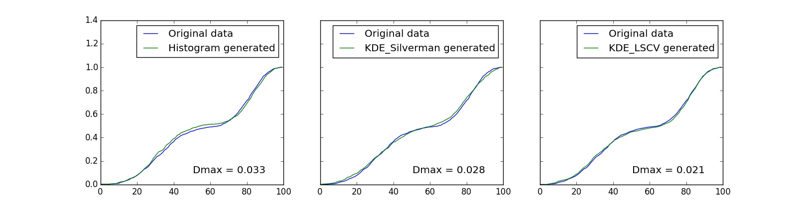
The above graphs shows us that the minimal difference D is using KDE method, where bandwidth is found using least squares cross validation. To check the hypothesis that newly generated data has the same distribution as original we use the following code below. There is a deep theory explanation why such values as in the code defines the limit to accept the hypothesis, but we do not dig into it this article.

lenGenerated=1000
for D in (DHist,DKDE_Silverman,DKDE_LSCV):
    if D>1.36*np.sqrt((lenDataset+lenGenerated)/(1.0*lenDataset*lenGenerated)):
        print ("Null hypothesis rejected")
    else:
        print ("Same distribution")

Download Scripts And Dataset

The code and dataset used in the tutorial are located on GitHub.