
Excel: Pivot Table Text Value Instead of Counts For Sub-group Listings
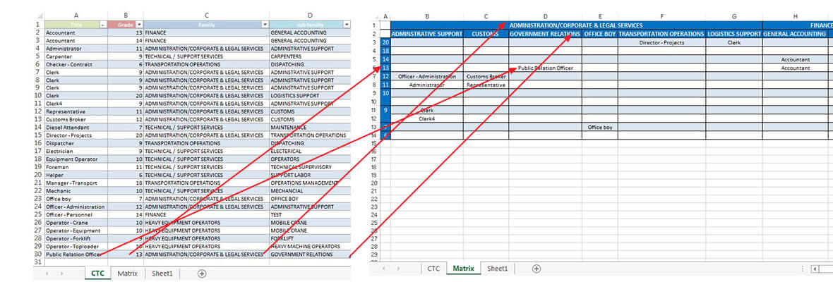
Task: Format data to a table in such a way that categories are columns and grouped text values are distributed by group numbers (take a look at Data and Results images below to grasp the idea).
Method: Pivot table, VBA
Requirements: Microsoft Excel 2007 or higher
Data and Results:


Contents:
Intro
It is a few stages process to create the resulting table from data. Everything will be included in VBA, but the main steps are these:
- Create Pivot Table and add filters
- Copy Pivot Table into new sheet
- Use for cycles to replace numbers with text
- Format final table
Create Pivot Table and Add Filters
Step 1: Create new sheet, Insert -> Pivot Table. Set range of Data to CTC!$A:$D.
Step 2: Set Pivot Table fields like it is shown below. Press on sub family and filter out blanks.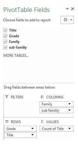
Step 3: In Excel tabs choose Design -> Subtotals -> Do not show Subtotals.
In Excel tabs choose Design -> Grand Totals -> Do not show Grand Totals.
To show row labels side-by side press on any grade number -> Excel tab Analyze -> Active Field -> Field Settings -> Layout and Print -> check Show item labels in tabular form.
Right Click anywhere on PivotTable. Choose PivotTable options. Set Merge cells with labels on.
Step 4: Make sure your table is called PivotTable1 and it is placed on Sheet1. Otherwise you will have to edit VBA a bit.
Step 5: Create button on CTC Sheet and assign VBA to it.
VBA Part Of The Task
For many non-programmers this part might be challenging, but by going line-by-line you should get the point. There are four VBA functions used:
Macro1_UpdateAndCopy() - It removes the result sheet if it exists, copies PivotTable and pastes it in the resulting sheet called "Matrix". Then it calls for the second macro.
1 2 3 4 5 6 7 8 9 10 11 12 13 14 15 16 17 18 19 20 21 22 23 24 25 26 27 28 29 30 31 32 33 34 35 36 37 38 39 40 41 42 43 44 45 46 | Sub Macro1_UpdateAndCopy() Application.DisplayAlerts = False Dim pt As PivotTable Set pt = Sheets("Sheet1").PivotTables("PivotTable1") pt.RefreshTable Sheets("Sheet1").Select 'Create sheet for results or delete existing and create Dim sh As Worksheet, flg As Boolean For Each sh In Worksheets If sh.Name Like "Matrix" Then flg = True: Exit For Next If flg = True Then Sheets("Matrix").Select ActiveWindow.SelectedSheets.Delete Sheets.Add.Name = "Matrix" Else Sheets.Add.Name = "Matrix" End If 'Copy Pivot Sheets("Sheet1").Select Dim LastRow As Long With ActiveSheet LastRow = .Range("A1").SpecialCells(xlCellTypeLastCell).Row End With Dim LastColumn As Long With ActiveSheet LastColumn = .Range("A1").SpecialCells(xlCellTypeLastCell).Column End With Range(Cells(1, 1), Cells(LastRow, LastColumn)).Select Selection.Copy Sheets("Matrix").Select Cells(1, 1).Select Selection.PasteSpecial Paste:=xlPasteValues, Operation:=xlNone, SkipBlanks _ :=False, Transpose:=False Application.DisplayAlerts = True Call Macro2_InsertText End Sub |
Macro2_InsertText() - It replaces count values in pivot table by text at the left in the beginning on the same row, then calls for next macro.
1 2 3 4 5 6 7 8 9 10 11 12 13 14 15 16 17 18 19 20 21 22 23 24 25 26 27 28 29 30 31 32 33 34 35 36 37 38 39 40 41 | Sub Macro2_InsertText() Dim LastRow As Long With ActiveSheet LastRow = .Range("B1").SpecialCells(xlCellTypeLastCell).Row End With Dim LastColumn As Long With ActiveSheet LastColumn = .Range("A1").SpecialCells(xlCellTypeLastCell).Column End With Range(Columns(1), Columns(LastColumn)).Select With Selection .HorizontalAlignment = xlCenter .VerticalAlignment = xlBottom .WrapText = False .Orientation = 0 .AddIndent = False .IndentLevel = 0 .ShrinkToFit = False .ReadingOrder = xlContext .MergeCells = False End With Dim a For irow = 4 To LastRow a = Cells(irow, 2).Value For icol = 3 To LastColumn If (Cells(irow, icol).Value > 0) Then Cells(irow, icol).Value = a End If Next icol Next irow Columns("B").EntireColumn.Delete Columns("A:AZ").EntireColumn.AutoFit Call Macro3_FitTable End Sub |
Sub Macro3_FitTable() - Removes unnecessary/empty rows and calls for next macro.
1 2 3 4 5 6 7 8 9 10 11 12 13 14 15 16 17 18 19 20 21 22 23 24 25 26 27 28 29 30 31 32 33 34 35 36 37 38 39 40 41 42 43 44 45 46 47 48 49 50 | Sub Macro3_FitTable() Dim LastRow As Long With ActiveSheet LastRow = .Range("B1").SpecialCells(xlCellTypeLastCell).Row End With Dim LastColumn As Long With ActiveSheet LastColumn = .Range("A1").SpecialCells(xlCellTypeLastCell).Column End With Dim b, temp b = 0 Dim groupRowNum For i = 4 To LastRow If Cells(i, 1) <> b And Cells(i, 1) > 0 Then b = Cells(i, 1) groupRowNum = i GoTo skipLoop End If temp = groupRowNum For icol = 2 To LastColumn If Cells(i, icol) <> 0 Then Do While temp < i If Cells(temp, icol) = 0 Then Cells(temp, icol).Value = Cells(i, icol) Cells(i, icol) = "" temp = i GoTo endLoop Else temp = temp + 1 End If endLoop: Loop End If Next icol skipLoop: Next i deletedRows = 0 For x = LastRow To 1 Step -1 If Application.WorksheetFunction.CountA(Rows(x)) = 0 Then Rows(x).Select Selection.Delete Shift:=xlUp deletedRows = deletedRows + 1 End If Next x Call Macro4_MergeAndColor(LastRow - deletedRows) End Sub |
Macro4_MergeAndColor - simply merges and colors the table.
1 2 3 4 5 6 7 8 9 10 11 12 13 14 15 16 17 18 19 20 21 22 23 24 25 26 27 28 29 30 31 32 33 34 35 36 37 38 39 40 41 42 43 44 45 46 47 48 49 50 51 52 53 54 55 56 57 58 59 60 61 62 63 64 65 66 67 68 69 70 71 72 73 74 75 76 77 78 79 80 81 82 83 84 85 86 87 88 89 90 91 92 93 94 95 96 97 98 99 100 101 102 103 104 105 106 107 108 109 110 111 112 113 114 115 116 117 118 119 120 121 122 123 124 125 126 127 128 129 130 131 132 133 134 135 136 137 138 | Sub Macro4_MergeAndColor(LastRow As Long) Cells(1, 1).Value = "" Dim LastColumn As Long With ActiveSheet LastColumn = .Range("A3").SpecialCells(xlCellTypeLastCell).Column End With Range(Cells(4, 1), Cells(LastRow, 1)).Select With Selection.Font .Name = "Calibri" .Size = 12 .Strikethrough = False .Superscript = False .Subscript = False .OutlineFont = False .Shadow = False .Underline = xlUnderlineStyleNone .ThemeColor = xlThemeColorDark1 .TintAndShade = 0 .ThemeFont = xlThemeFontMinor End With With Selection.Interior .Pattern = xlSolid .PatternColorIndex = xlAutomatic .Color = 12611584 .TintAndShade = 0 .PatternTintAndShade = 0 End With Range(Cells(2, 2), Cells(3, LastColumn - 1)).Select With Selection.Interior .Pattern = xlSolid .PatternColorIndex = xlAutomatic .ThemeColor = xlThemeColorDark2 .TintAndShade = -9.99786370433668E-02 .PatternTintAndShade = 0 End With Range(Cells(2, 1), Cells(LastRow, LastColumn - 1)).Select With Selection.Borders(xlInsideHorizontal) .LineStyle = xlContinuous .ColorIndex = 0 .TintAndShade = 0 .Weight = xlThin End With 'merge Groups vallindex = 4 For ind = 5 To LastRow If Cells(ind, 1) < 1 Then Range(Cells(vallindex, 1), Cells(ind, 1)).Select Selection.Merge With Selection .HorizontalAlignment = xlCenter .VerticalAlignment = xlTop .WrapText = False .Orientation = 0 .AddIndent = False .IndentLevel = 0 .ShrinkToFit = False .ReadingOrder = xlContext .MergeCells = True End With End If vallindex = ind Next ind 'merge Family vallindex = 2 For ind = 3 To LastColumn - 1 If Cells(2, ind) < 1 Then Range(Cells(2, vallindex), Cells(2, ind)).Select Selection.Merge With Selection .HorizontalAlignment = xlCenter .VerticalAlignment = xlTop .WrapText = False .Orientation = 0 .AddIndent = False .IndentLevel = 0 .ShrinkToFit = False .ReadingOrder = xlContext .MergeCells = True End With End If vallindex = ind Next ind Range(Cells(1, 1), Cells(LastRow, LastColumn - 1)).Select Selection.Borders(xlDiagonalDown).LineStyle = xlNone Selection.Borders(xlDiagonalUp).LineStyle = xlNone With Selection.Borders(xlEdgeLeft) .LineStyle = xlContinuous .ColorIndex = 0 .TintAndShade = 0 .Weight = xlThin End With With Selection.Borders(xlEdgeTop) .LineStyle = xlContinuous .ColorIndex = 0 .TintAndShade = 0 .Weight = xlThin End With With Selection.Borders(xlEdgeBottom) .LineStyle = xlContinuous .ColorIndex = 0 .TintAndShade = 0 .Weight = xlThin End With With Selection.Borders(xlEdgeRight) .LineStyle = xlContinuous .ColorIndex = 0 .TintAndShade = 0 .Weight = xlThin End With With Selection.Borders(xlInsideVertical) .LineStyle = xlContinuous .ColorIndex = 0 .TintAndShade = 0 .Weight = xlThin End With With Selection.Borders(xlInsideHorizontal) .LineStyle = xlContinuous .ColorIndex = 0 .TintAndShade = 0 .Weight = xlThin End With Cells(1, 1).Select End Sub |
Download The Code
In the given Excel file just click "UPDATE" on CTC sheet and watch it happen. The code and example Excel file are available on GitHub.